Automagic Tabs in Distill/Rmarkdown files and time series analysis

This article shows the use of tabs in Rmarkdown documents, through an example of time series analysis of the monthly estimator of Argentine economic activity.

Tidy tabs approach 🧙

When conducting exploratory data analysis 📈, reporting on models 🤖, or simply presenting results obtained, we usually have dozens of plots to show. For this reason, it is necessary to organize the report in a way to focus the reader’s attention on certain aspects and not overwhelm them with all the information at once.

👉 We use a Tidy approach to generate tabs in automated format from a nested tibble that contains the objects to include in each tab.

This article is based on a previous article we’ve written on time series analysis: Multiple models on multiple time series: A Tidy approach.

Libraries 📚

The necessary libraries are imported. sknifedatar

Zambrano and Bartolome (2021)

¹ is a package that serves primarily as an extension to the modeltime 📦 ecosystem, in addition to some functionalities of spatial data and visualization. In this case, we are going to use the automagic_tabs function from this package.

For data manipulation we used the tidyverse

Wickham et al. (2019)

² ecosystem.

library(sknifedatar)

#devtools::install_github("gadenbuie/xaringanExtra")
library(xaringanExtra)

library(lubridate)
library(timetk)
library(dplyr)
library(tidyr)
library(purrr)
library(reactable)
library(htmltools)

What are tabs? 🤔

✏️ A tab is a design pattern where content is separated into different panes, and each pane is viewable one at a time.

• 👋 Hey!
• Unsolicited advice 1
• Unsolicited advice 2
• Unsolicited advice 3
• 🔚 Ending tab

This is tab number 1 . 🌟 Check the following tabs for some unsolicited advice 🌟 👆

This is tab number 2

This is tab number 3

This is tab number 4

This is tab number 5. Thank you for reading this far.

How to generate tabs? 🗂️

🔹 In order to generate the tabs above, the following chunks were necessary:

Show code

# ::: {.l-page}
# ::: {.panelset}
# ::: {.panel}
# ## 👋 Hey! {.panel-name}
# 
# This is tab number 1 . 🌟 [**Check the following tabs for some unsolicited advice**]{.ul} 🌟 👆
# :::
# 
# ::: {.panel}
# ## Unsolicited advice 1 {.panel-name}
# 
# This is tab number 2
# 
# ```{r, out.width="50%",echo=FALSE ,fig.align = 'center'}
# knitr::include_graphics('https://media.tenor.com/images/be8a87467b75e9deaa6cfe8ad0b739a0/tenor.gif')
# ```
# :::
# 
# ::: {.panel}
# ## Unsolicited advice 2 {.panel-name}
# 
# This is tab number 3
# 
# ```{r, out.width="50%",echo=FALSE ,fig.align = 'center'}
# knitr::include_graphics('https://media.tenor.com/images/6a2cca305dfacae61c5668dd1687ad55/tenor.gif')
# ```
# :::
# 
# ::: {.panel}
# ## Unsolicited advice 3 {.panel-name}
# 
# This is tab number 4
# 
# ```{r, out.width="50%",echo=FALSE ,fig.align = 'center'}
# knitr::include_graphics('https://media.tenor.com/images/bfde5ad652b71fc9ded82c6ed760355b/tenor.gif')
# ```
# :::
# 
# ::: {.panel}
# ## 🔚 Ending tab {.panel-name}
# 
# This is tab number 5. Thank you for reading this far.
# 
# ```{r, out.width="50%",echo=FALSE ,fig.align = 'center'}
# knitr::include_graphics('https://media.tenor.com/images/3f9ea6897492ac63d0c46eb53ae79b11/tenor.gif')
# ```
# :::
# :::
# :::

🔎 As it can be seen, this is not so difficult. However, what if we wanted to generate 16 tabs instead of 4?

Using a tidy approach, an automatic tab generation 🧙 can be performed by nesting the objects to include in each tab. Let’s see an example.

Data 📊

For this example, time series data from the Argentine monthly economic activity estimator (EMAE) is used. This data is available in the sknifedatar package 📦.

emae <- sknifedatar::emae_series 

Nested dataframes 📂

🔹 The first step is to generate a nested data frame. It includes a row per economic sector.

nest_data <- emae %>%
  nest(nested_column = -sector)

nest_data

# A tibble: 16 x 2
   sector                           nested_column     
   <chr>                            <list>            
 1 Comercio                         <tibble [202 × 2]>
 2 Ensenanza                        <tibble [202 × 2]>
 3 Administracion publica           <tibble [202 × 2]>
 4 Transporte y comunicaciones      <tibble [202 × 2]>
 5 Servicios sociales/Salud         <tibble [202 × 2]>
 6 Impuestos netos                  <tibble [202 × 2]>
 7 Sector financiero                <tibble [202 × 2]>
 8 Mineria                          <tibble [202 × 2]>
 9 Agro/Ganaderia/Caza/Silvicultura <tibble [202 × 2]>
10 Electricidad/Gas/Agua            <tibble [202 × 2]>
11 Hoteles/Restaurantes             <tibble [202 × 2]>
12 Inmobiliarias                    <tibble [202 × 2]>
13 Otras actividades                <tibble [202 × 2]>
14 Pesca                            <tibble [202 × 2]>
15 Industria manufacturera          <tibble [202 × 2]>
16 Construccion                     <tibble [202 × 2]>

👀 To better understand the format of nest_data, the "nested_column" variable is disaggregated below. By clicking on each sector, it can be seen that 👉👉 each nested column includes data for the series of the selected sector. In the first row, data corresponds to the monthly activity estimator from 2004-01-01 to 2020-10-01 for the ‘Commerce’ sector.

Show code

reactable(nest_data, details = function(index) {
  data <- emae[emae$sector == nest_data$sector[index], c('date','value')] %>% 
    mutate(value = round(value, 2))
  div(style = "padding: 16px",
                 reactable(data, outlined = TRUE)
  )
}, defaultPageSize=5)

sector

nested_column

•​

Comercio

[object Object]

•​

Ensenanza

[object Object]

•​

Administracion publica

[object Object]

•​

Transporte y comunicaciones

[object Object]

•​

Servicios sociales/Salud

[object Object]

1–5 of 16 rows

Previous1234Next

The above interactive table was made using reactable

Lin (2020)

³ and htmltools

Cheng et al. (2021)

⁴ .

📌 Note that when extracting the nested_column from the first row, the data corresponding to the series of the first sector is obtained.

nest_data %>% pluck("nested_column",1)

date

value

2004-01-01

92.0653378369893

2004-02-01

91.4647184549155

2004-03-01

109.127779788592

2004-04-01

99.4201409563252

2004-05-01

100.53274443267

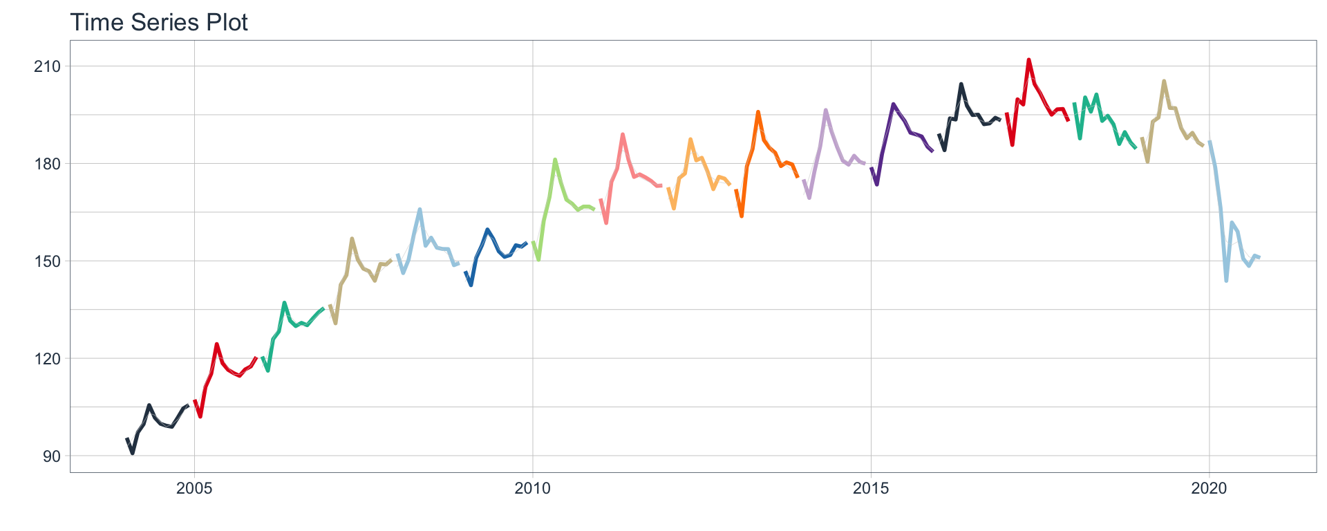
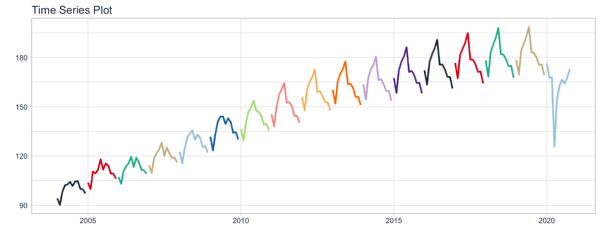
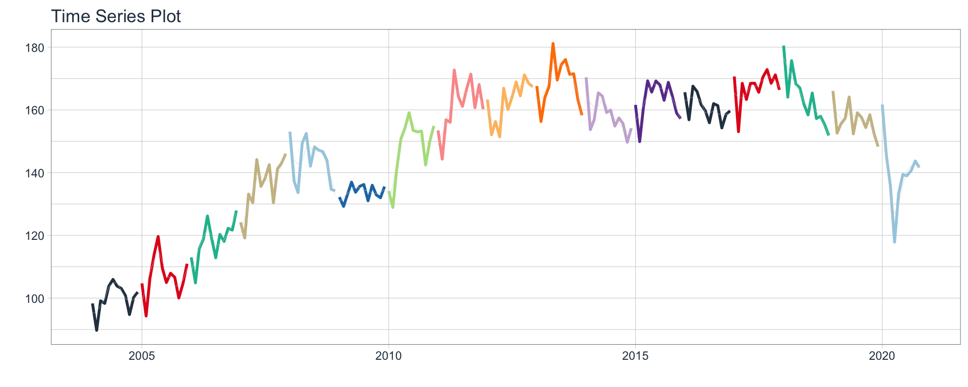
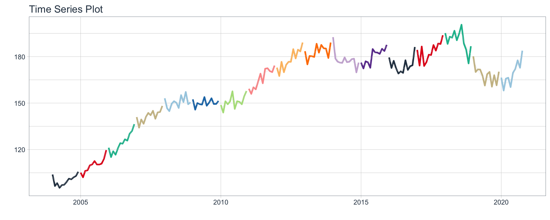
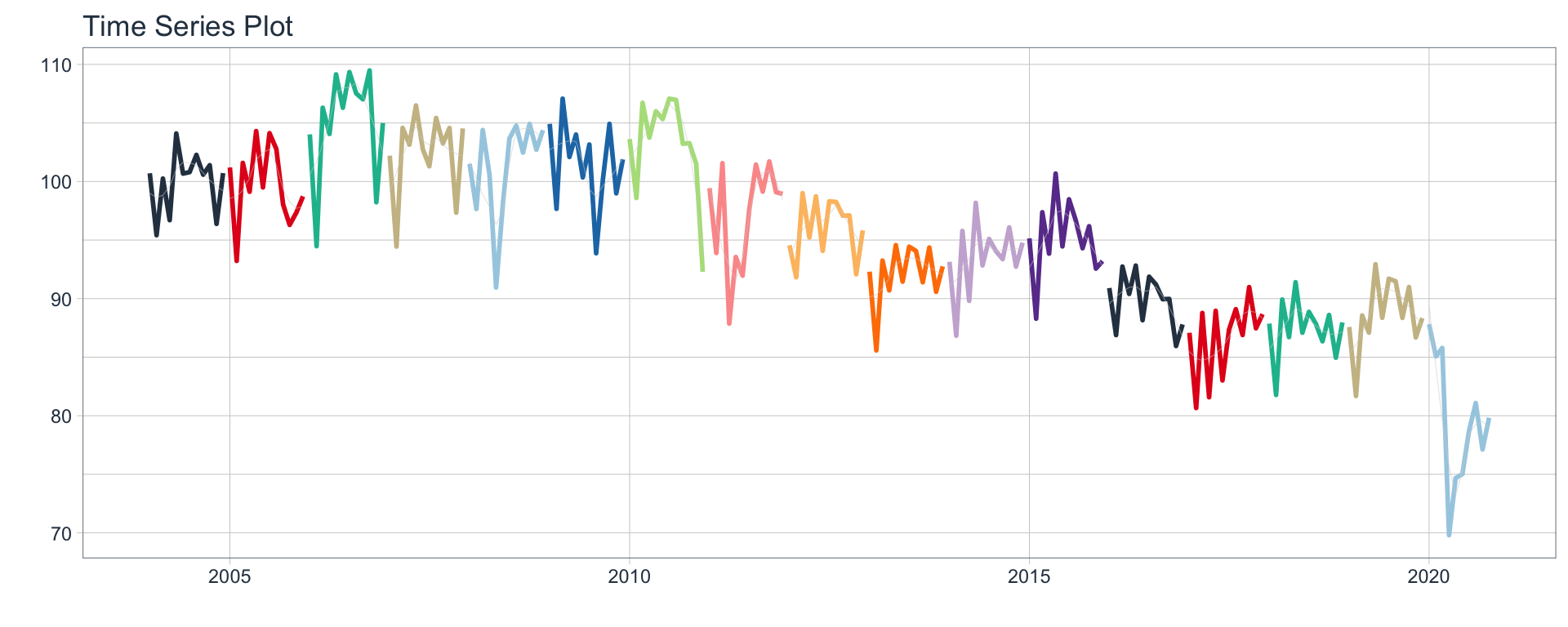
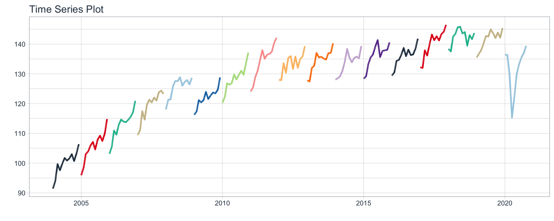
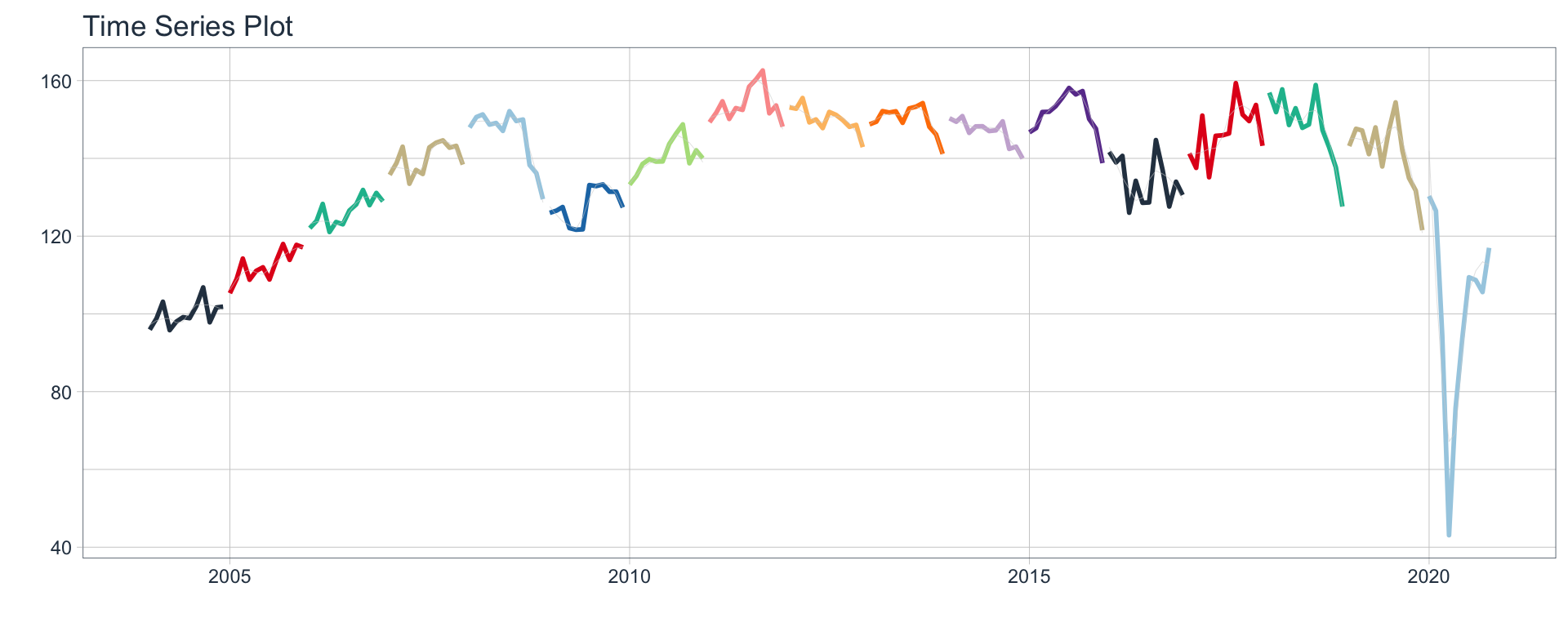
Time series plots 🌠

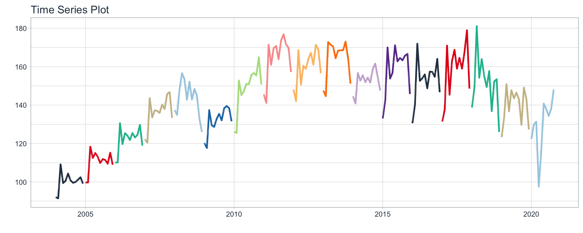
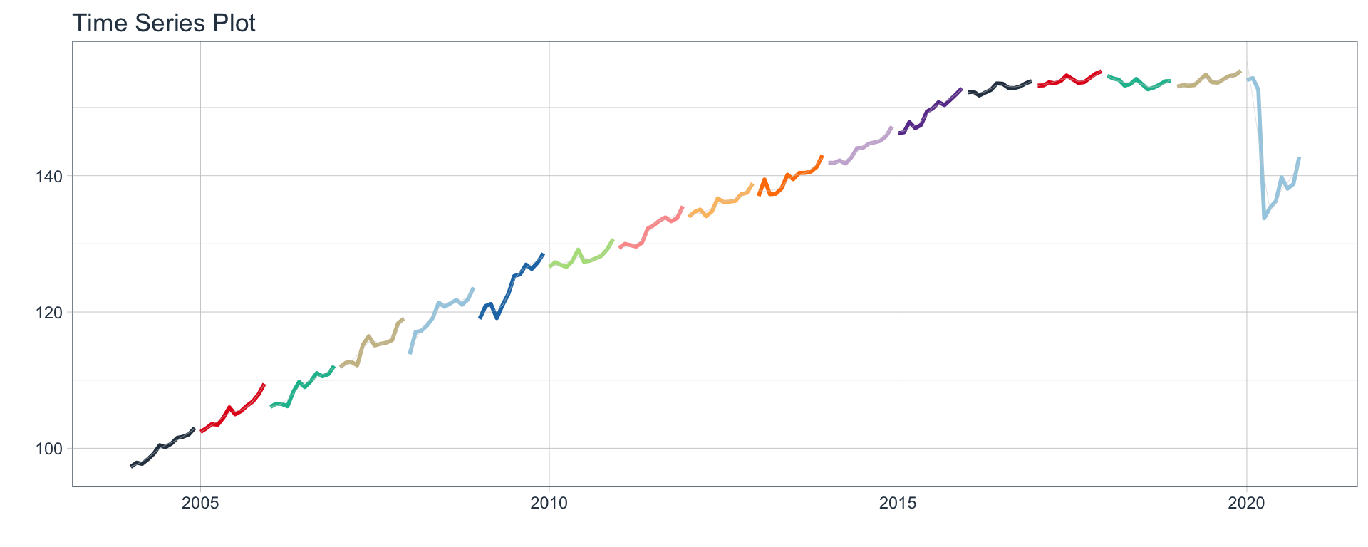
👉 The evolution of each series can be observed by using a tab for each sector. This allows the visualization to be much clearer 🙌, allowing the reader to focus on each series, without having to view multiple plots of the same type.

nest_data <- 
  nest_data %>%
  mutate(ts_plots = map(nested_column, 
                        ~ plot_time_series(.data = .x,
                                           .date_var = date,
                                           .value = value,
                                           .color_var = year(date),
                                           .interactive = FALSE,
                                           .line_size = 1, 
                                           .smooth_color = 'lightgrey',
                                           .smooth_size = 0.1,
                                           .legend_show = FALSE
                                          )))
nest_data

# A tibble: 16 x 3
   sector                           nested_column      ts_plots
   <chr>                            <list>             <list>  
 1 Comercio                         <tibble [202 × 2]> <gg>    
 2 Ensenanza                        <tibble [202 × 2]> <gg>    
 3 Administracion publica           <tibble [202 × 2]> <gg>    
 4 Transporte y comunicaciones      <tibble [202 × 2]> <gg>    
 5 Servicios sociales/Salud         <tibble [202 × 2]> <gg>    
 6 Impuestos netos                  <tibble [202 × 2]> <gg>    
 7 Sector financiero                <tibble [202 × 2]> <gg>    
 8 Mineria                          <tibble [202 × 2]> <gg>    
 9 Agro/Ganaderia/Caza/Silvicultura <tibble [202 × 2]> <gg>    
10 Electricidad/Gas/Agua            <tibble [202 × 2]> <gg>    
11 Hoteles/Restaurantes             <tibble [202 × 2]> <gg>    
12 Inmobiliarias                    <tibble [202 × 2]> <gg>    
13 Otras actividades                <tibble [202 × 2]> <gg>    
14 Pesca                            <tibble [202 × 2]> <gg>    
15 Industria manufacturera          <tibble [202 × 2]> <gg>    
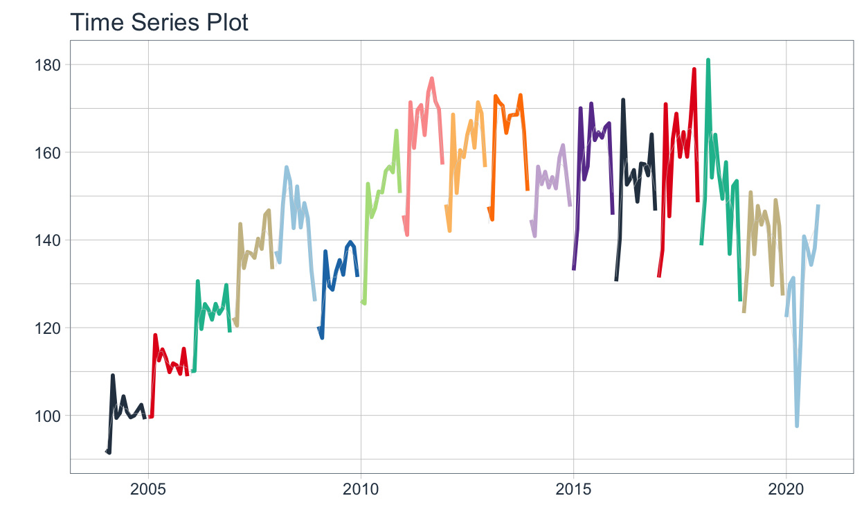
16 Construccion                     <tibble [202 × 2]> <gg>    

📽 First, a column called “ts_plots” is added, where we store the visualizations of the time series. For this we apply the function “plot_time_series” on each series stored in the column “nested_column” through the function "map". The function plot_time_series is included on the timetk

Dancho and Vaughan (2021)

⁵ package 📦. One of the series is displayed below.Notice that we are using lubridate

Grolemund and Wickham (2011)

⁶ package to add different colors for each year. This allows us to infer if seasonality is present in each time series, although we will analyse this later on this article.

nest_data %>% pluck("ts_plots",1)

Perfect, but … if we wanted to graph all the time series, how could we do it? 🤔

The “automagic_tabs” function of the sknifedatar package was created for this. It receives 3 main arguments:

• input_data: The nested dataframe that we have created 💾, in our case, the “nest_data” object.

• panel_name: The name of the column of the nested dataframe where the series names are, these names will be the titles of each tabs 📝. In our case, “sector.”

• .output: The name of the column of the nested dataframe that stores the graphs to be displayed 📈. In our case, “ts_plots.”

🛠 Additional arguments: you can specify the width of the set of panels in “.layout,” 👉👉👉 in addition to being able to specify all the parameters available on rmarkdown chunks 🙌 (fig.align, fig.width, …)

🔹 Let’s see the application below, first we invoke the “use_panelset" function from the xaringanExtra

Aden-Buie (2021)

⁷ package 📦 and then the”automagic_tabs" function.

xaringanExtra::use_panelset()

`r automagic_tabs(input_data = nest_data, panel_name = "sector", .output = "ts_plots",
                  .layout = "l-page", fig.heigth=1, fig.width=10)`

• Comercio
• Ensenanza
• Administracion publica
• Transporte y comunicaciones
• Servicios sociales/Salud
• Impuestos netos
• Sector financiero
• Mineria
• Agro/Ganaderia/Caza/Silvicultura
• Electricidad/Gas/Agua
• Hoteles/Restaurantes
• Inmobiliarias
• Otras actividades
• Pesca
• Industria manufacturera
• Construccion

⚠ Note something important, 👉👉👉 the function does not run in a chunk, it is invoked “inline” (or an r function between apostrophes) within the Rmarkdown document. Below is the complete code:

#---
#title: "automagic_tabs"
#author: "sknifedatar"
#output: html_document
#---
#
#```{r}
#library(sknifedatar)
#library(timetk)
#```
#
#```{r}
#emae <- sknifedatar::emae_series 
#
#nest_data <- emae %>%
#  nest(nested_column = -sector) %>% 
#  mutate(ts_plots = map(nested_column, 
#                        ~ plot_time_series(.data = .x,
#                                           .date_var = date,
#                                           .value = value,
#                                           .interactive = FALSE,
#                                           .line_size = 0.15)
#                         ))
#```
#
#```{r}
#xaringanExtra::use_panelset()
#```
#
#`r automagic_tabs(input_data = nest_data, panel_name = "sector", .output = "ts_plots")`

🔹 Copy the code above, paste it into a new Rmarkdown file, and hit knit the document to get the tabs.

Decomposition and autocorrelation 💡

Below is a brief exploratory analysis 💫 of 4 of the series, including decomposition and autocorrelation analysis. The results are presented in tabs, one for each sector for each type of analysis.

🔹 First we filter 4 series and add emojis to their names 😂.

data_filter <- 
  nest_data %>%
  filter(sector %in% c(
    'Mineria',
    'Industria manufacturera',
    'Pesca',
    'Construccion'
  )) %>% 
  mutate(
    sector = case_when(
      sector == 'Industria manufacturera' ~ 'Industria manufacturera ⚙️',
      sector == 'Pesca' ~ 'Pesca 🐠',
      sector == 'Construccion' ~ 'Construccion 🏠',
      sector == 'Mineria' ~ 'Mineria 🏔'
    )) %>% 
  arrange(sector)
  
data_filter 

# A tibble: 4 x 3
  sector                     nested_column      ts_plots
  <chr>                      <list>             <list>  
1 Construccion 🏠            <tibble [202 × 2]> <gg>    
2 Industria manufacturera ⚙️ <tibble [202 × 2]> <gg>    
3 Mineria 🏔                 <tibble [202 × 2]> <gg>    
4 Pesca 🐠                   <tibble [202 × 2]> <gg>    

🔹 Now the decomposition plots are added in the STL column. This is later plotted with the function automagic_tabs.

data_filter <- data_filter %>%
  mutate(ACF = map(nested_column, 
                   ~ plot_acf_diagnostics(.data = .x, date, value,
                                          .show_white_noise_bars = TRUE,
                                          .white_noise_line_color = 'red',
                                          .white_noise_line_type = 2,
                                          .line_size = 0.4,
                                          .point_size = 0.7,
                                          .interactive = FALSE))) 

📌 STL plots contain 4 nested graphs, therefore we will increase the height of the figure to 8 and change the layout.

`r automagic_tabs(input_data=data_filter ,panel_name="sector",.output="ACF" ,
                  fig.height=5 ,.layout="l-body-outset")`

• Construccion 🏠
• Industria manufacturera ⚙️
• Mineria 🏔
• Pesca 🐠

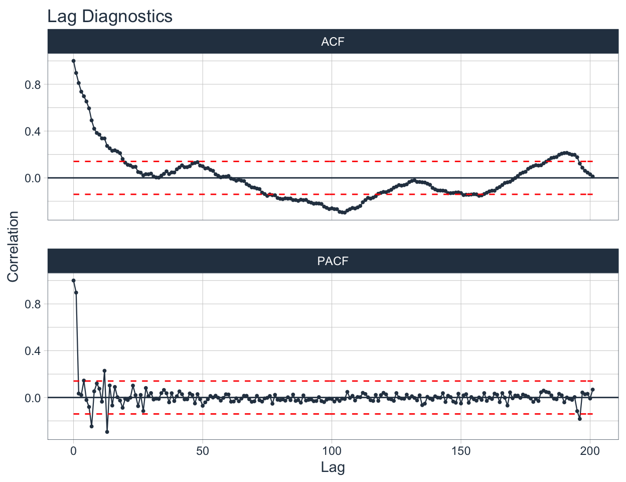
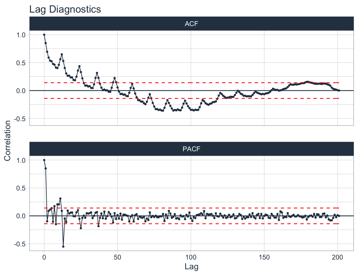
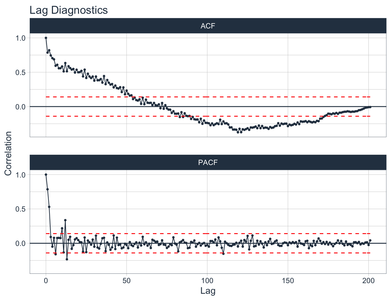
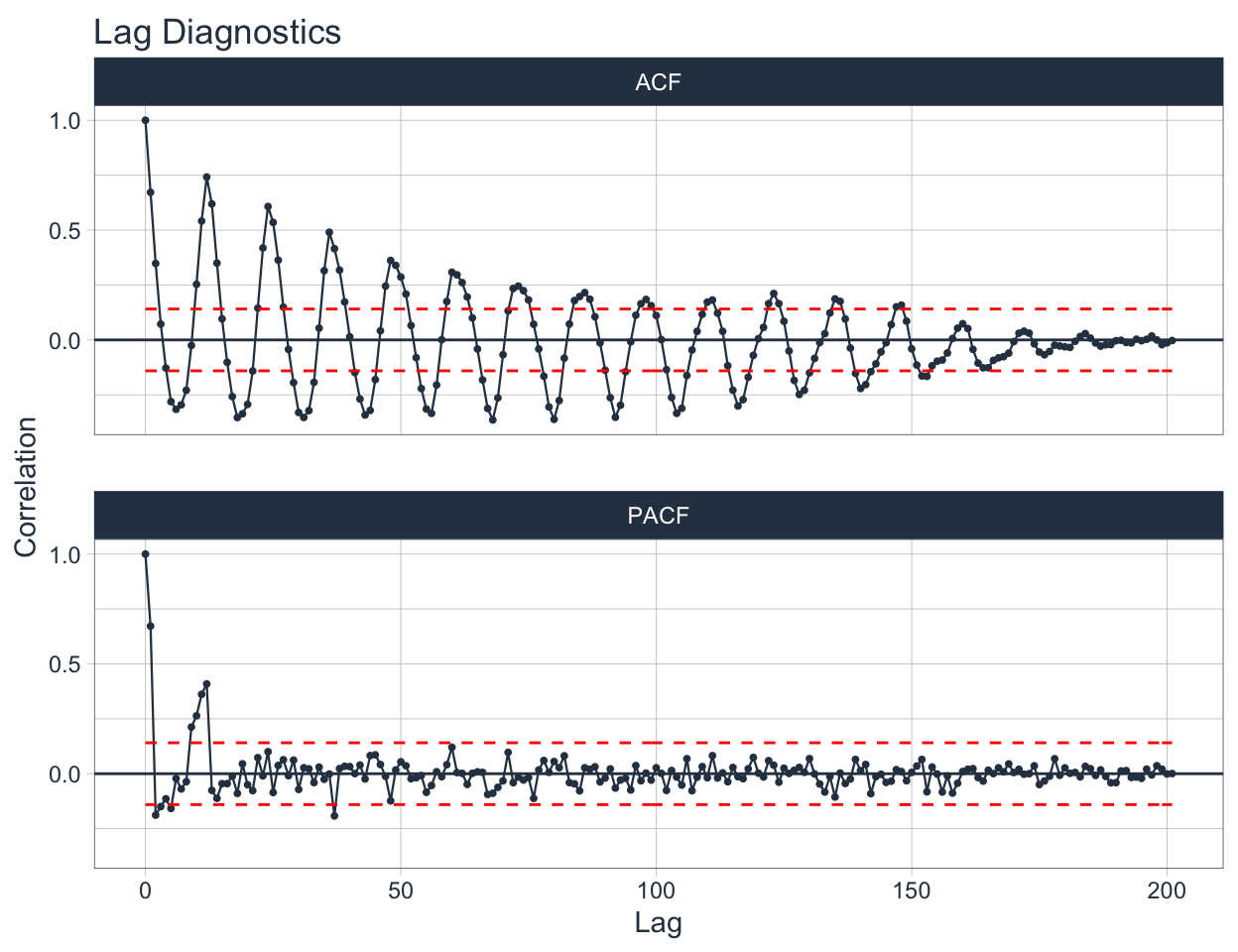
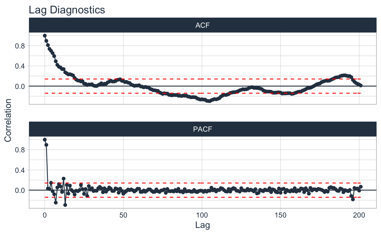
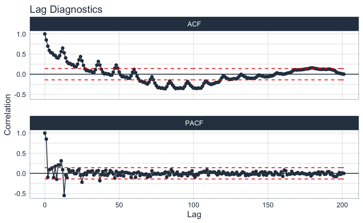
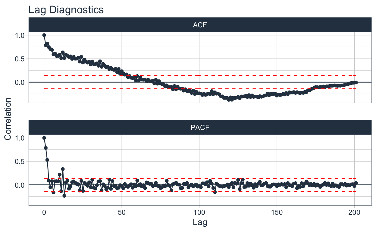
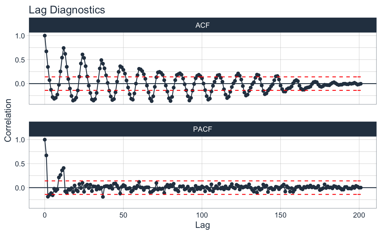
🔹 Finally the autocorrelation plots are added in the ACF column. This is also plotted on tabs with the automagic_tabs function.

data_filter <- data_filter %>%
  mutate(ACF = map(
    nested_column, 
    ~ plot_acf_diagnostics(.data = .x, date, value,
                           .show_white_noise_bars = TRUE,
                           .white_noise_line_color = 'red',
                           .white_noise_line_type = 2,
                           .line_size = 0.5,
                           .point_size = 1.5,
                           .interactive = FALSE
                        )
  )) 

data_filter 

# A tibble: 4 x 4
  sector                     nested_column      ts_plots ACF   
  <chr>                      <list>             <list>   <list>
1 Construccion 🏠            <tibble [202 × 2]> <gg>     <gg>  
2 Industria manufacturera ⚙️ <tibble [202 × 2]> <gg>     <gg>  
3 Mineria 🏔                 <tibble [202 × 2]> <gg>     <gg>  
4 Pesca 🐠                   <tibble [202 × 2]> <gg>     <gg>  

`r automagic_tabs(input_data = data_filter , panel_name = "sector", .output = "ACF",
                  .layout="l-body-outset")`

• Construccion 🏠
• Industria manufacturera ⚙️
• Mineria 🏔
• Pesca 🐠

The emojis are displayed in the tab titles 🤩🤩🤩.

Thank you very much for reading us 👏👏👏.

Contacts ✉

Karina Bartolome, Linkedin, Twitter, Github, Blogpost.

Rafael Zambrano, Linkedin, Twitter, Github, Blogpost.